Biology embodies chaotic process in many areas, from plant-like fractals to mathematical models of populations and predator-prey systems. Genetics, aspects of human biology, and many rhythmic behaviours of nature are also explainable through chaos theory.
For ecologists and biologists, population studies frequently play an important role. Examining a population mathematically can be a useful tool, allowing current populations to be understood and future populations to be predicted. Mathematically, populations can be viewed as feedback loops; this years population impacts directly on that of the following year. Finding an equation that matches a real life scenario is incredibly difficult there are so many factors to take into consideration. For example, a species can be affected by many predators, various food and habitat requirements (each of which depend on equally complex requirements). It is not enough to know that birds eat moths, it is also necessary to know at what rate this occurs.
Since nature is highly complex, ecologists look to simplified mathematical
models as a means of approximation. These approximations measure population
growth in regular intervals, not on a continual basis. The simplest of
these imagines a world with infinite resources (food, habitat, etc) and
no predators. The population increases like a compound interest sum, growing
exponentially. Such an equation is as follows: xnext = lx,
where l (lambda) is the rate of growth and x
represents the population. If x takes on a value of 0.4 and l
takes on a value of 2 then:
| X0 = 0.4 |
| X1 = 0.8 |
| X2 = 1.6 |
| X3 = 3.2 |
| X4 = 6.4 |
| X¥= ¥ |
This equation, the Malthusian model, is a poor demonstration of the natural world, and its shortcomings are pretty obvious. The world is not a place of infinite resource, so the next task is to add a limit factor to the equation, representing the maximum size of the population. The following equation is still highly simplistic, but does solve the
aforementioned problem: xnext = lx(1-x),
where x < 1 and l is the rate of growth.
In this equation, the population is scaled between 0 and 1. (1-x) adds
a limit to the population because as x rises, (1-x) falls accordingly.
In this model, if x takes on a value of 0.4 and l
a value of 2 then:
| X0 = 0.4 |
| X1 = 0.48 |
| X2 = 0.4992 |
| X3 = 0.4999987 |
| X4 = 0.5 |
| X5 = 0.5 |
The population has risen steeply to a state of equilibrium and settled
to a constant value of 0.5. As the value of l rises,
the population behaves in similar fashion, but reaches a higher equilibrium.
Here, l takes the value 2.3:
| X0 = 0.4 | X8 = 0.5652201 |
| X1 = 0.552 | X9 = 0.5652166 |
| X2 = 0.5687808 | X10 = 0.5652176 |
| X3 = 0.5641192 | X11 = 0.5652173 |
| X4 = 0.5655441 | X12 = 0.5652174 |
| X5 = 0.5651191 | X13 = 0.5652174 |
| X6 = 0.5652468 | X14 = 0.5652174 |
| X7 = 0.5652086 | X15 = 0.5652174 |
Moreover, as lambda increases still further, the population no longer
settles to a single number but begins to repeat in a series of two. l=
1 + 51/2 (» 3.236067977
):
| X0 = 0.4 | X8 = 0.5000874 |
| X1 = 0.7766563 | X9 = 0.809017 |
| X2 = 0.5613325 | X10 = 0.5 |
| X3 = 0.7968440 | X11 = 0.809017 |
| X4 = 0.5238665 | X12 = 0.5 |
| X5 = 0.8071737 | X13 = 0.809017 |
| X6 = 0.5036755 | X14 = 0.5 |
| X7 = 0.8089733 | X15 = 0.809017 |
Increasing lambda further, the pattern becomes more complicated. Rather than a series of two, the x repeats in a series of four, then eight and so forth. This process of periodic doubling is known as a bifurcation. Bifurcations were first studied by Robert May (see section 4.5). Before May, people had been looking at each iterative equation separately and looking for patterns and predicability within it. Robert May took a different approach. He took the last repeating values of a particular lambda and graphed these points next to that of the previous lambda. This enabled him to view the entire equation, not just a small part of it.
This image shows Mays approach when x=.4, lambda increments = .0001, iterations (see appendix 2) = 5000, and plotted points = 50:
The above diagram shows this process of bifurcation. When the whole equation xnext = lx(1-x) is displayed, the areas of order and chaos can be clearly seen. Denser regions can be seen running through the chaotic regions, these show areas with a high population probability. Although the population could end up anywhere within the white area, the denser areas represent a mild form of order.
Regions of chaos in the diagram are periodically interrupted by regions of order, where the disordered mass suddenly reduces into an odd number of single lines, before dissipating into chaos once more. If these ordered areas are shown in greater detail, they are exact replicas of the first bifurcation. This shows a form of order that can be seen on different scales rather than on the same scale. The order cannot be seen on scale of time, but it can be seen on a scale of magnification. Although this idea only became popular with the advent of fractals, it is not entirely new. Similar ideas have been explored by mathematicians like Helge von Koch, who investigated the Koch curve, showing an infinite distance in a finite line. The Sierpinski triangle is another similar example (see section 5.2.1).
When l approaches greater values still, all
traces of order vanish and chaos ensues. Here l
= 4.
| X0 = 0.4 | X6 = 0.02546474 |
| X1 = 0.96 | X7 = 0.09927552 |
| X2 = 0.1536001 | X8 = 0.3576796 |
| X3 = 0.5200284 | X9 = 0.9189796 |
| X4 = 0.9983954 | X10 = 0.2978244 |
| X5 = 0.00640793 |
This process shows the hallmarks of a chaotic system. With low input, the system is orderly, with increased input, the system becomes complex and eventually chaotic.
5.1.2 Chaos Theory as a Modelling Tool
As well as being used in population modelling, chaos theory has also been used to describe other areas of biology, from the fractal-like structure of blood vessels and capillaries to many rhythmic systems found within nature. Research under way at the University of Newcastle in Australia suggests that linked oscillators, themselves exponents of chaotic principles, provide excellent models for such behaviour. From insects like glow worms and cicadas to rhythmically contracting tissues in the gastro-intestinal system, living things display a broad range of rhythmic activity, for which oscillators working on chaotic principles may provide the best explanation. Longer rhythmic behaviour can be seen in the plant kingdom, with the opening and closing of leaves and flowers. On a longer scale still are seasonal variation, ovulation, and predator-prey population growth. Nature provides much rhythmic synchronicity.
However, disrupting these cycles can lead to chaotic behaviour before order re-emerges, as Mohammad S. Imtiaz, of the University of Newcastle, explains: "One example is the membrane voltage recording from a freshly dissected stomach tissue. Initially these tissues produce a very non-coherent output. But as time goes on most of them slowly develop a regular rhythmic pattern. A possible explanation is that the cells become de-coupled in a tissue that has been dissected, a kind of mechanical trauma. Slowly as the tissue starts recovering, the cells start to communicate with each other and a rhythmic activity emerges. We are still working on this and it is still a mystery to a large extent."
He goes on to give another example, involving insulin-secreting cells. When a few insulin-secreting cells are isolated they do not produce clean, rhythmic behaviour. However, as soon as a number of them are grouped together, a clean synchronised activity emerges. Although the processes involved in this transition are still largely unclear, it appears that chaos of this form is a transitory behaviour.
One of the puzzles of genetics is how a seed can contain all the information needed for the growth of a huge tree. However, research in fractals has shown that images of infinite complexity can be created using random processes combined with a few very simple rules. The Sierpinski triangle (see section 5.2.1) is a good example. Similar rules can be used to generate more natural formations, and, as discovered by mathematician Michael Barnsley, of Georgia Institute of Technology, it is possible to find rules for objects in the natural world. Based on the principle that nature possesses self-similarity, Barnsley was able to create a rule that reproduced an exact replica of a black spleenwort fern that "no biologist would have any trouble identifying." Although the method, known as the collage theorem, is complicated, simple rules can be found for any of the many natural shapes that possess self-similarity.
While, evidence is inconclusive, Barnsley has, at least, made plausible the idea that plants store genetic information in a similar way.
The geometry of chaos theory requires computers, for the most part, to generate the highly complex images involved. Surprisingly, these images are generated using relatively simply iterative complex number equations.
Computer imagery has played a large part in chaos theorys appeal with the wider public, the colourful fractal images striking a cord with the laymans artistic sense.
Julia Sets, some of the earliest fractals to be explored, were first experimented with and discovered by the duo of Gaston Julia and Pierre Fatou (see section 4.2). Julia Sets are maps on a complex number plane. A complex number z contains two parts, a real part and an imaginary part. That is, z = x + iy, where x and y are real numbers and i is the imaginary nubmer, -11/2. When working with complex numbers, the real and imaginary parts are considered separately, as in normal algebra.
z2 = (x+iy)(x+iy)
= x2 + 2iyx + i2y2
= x2 + 2iyx y2
Julia Sets work with iterative equations, for example F(z) = z2. Z0 = x0 + iy0 with |z| <1. Iterating this equation moves it closer to zero. Thus, as long as 0<|z0|<1 then F(z) tends towards zero and consequently can be considered stable. If |z0| >1 then it follows that F(z) tends towards infinity and is considered unstable.
Julia Sets are defined by the iterative equation z = z2 + c and consists of all points that do not tend to infinity. Every Julia Set is characterised by a unique value of the complex constant c.
Julia Sets posses very similar properties to simple fractals such as the Koch curve, showing infinite complexity and self-similarity on differing scales.
Through experimentation with models of Julia Sets, it has been found in this study that altering the real and imaginary parts of z have differing impacts on the form of the image, as described below.
As soon as c is increased above 0 by even the smallest margin in either the real or imaginary part, the resulting image is of a near perfect circle. Hence, it is the starting image for the Julia Sets sequences displayed on the following pages. They are achieved by plotting a series of Julia Sets, increasing (or decreasing) either the real or imagery parts of the constant c by a set margin each time. For convenience, these are referred to in this study as sequential Julia Sets.
These images show the y value, or the imaginary part of the complex constant c, being increased (clockwise from top left) as follows: 0.25, 0.5, 0.75, 1. Decreasing the y value (ie 0.25, -0.5 etc) simply mirrors each image.
These images show the x value, or the real part of the complex constant c, being increased (clockwise from top left) as follows: 0.25, 0.5, 0.75, 1. Unlike with the y value, decreasing the x value results in a new set of images, shown below.
These images show the x value being decreased (clockwise from top left)
as follows:
-0.25, -0.5, -0.75, -1.
This image shows Julia Sets respective to their place in the complex number plane. The circular Julia Set in the centre shows x = 0.00001, y = 0. Extending out from it are Julia Sets at intervals of 0.5. Hence, the set in the bottom left hand corner shows
x = -1, y = -1. It clearly shows the transformation of sequential Julia Sets and the effects of the real and imaginary parts on the form of the image. The sets at 45 degrees to the x, y axis can be seen as a combination of their counterparts on the axis. For example, the set at (0.5, 0.5) is a combination of the sets at (0, 0.5) and (0.5, 0).
The above image shows 3-dimensional plotting of a sequential Julia Set. Each set is plotted on top of the previous, and hence, the method is able to show an entire sequential Julia Set simultaneously. Inspiration for this technique was drawn from Robert May (see section 4.5), who shed new light on bifurcations using a similar procedure. This set starts at (0,0) with the y value being increased by 0.001 for each of the 50,000 iterations.
Fractals can be used to create stunning visual landscapes with startling realism. Mandelbrot called it the geometry of nature for no insignificant reason. When looking at the world, Mandelbrot realised that much of the world around us cannot be explained by the traditional Euclidean geometry of spheres and cubes. As he said,
Each successively small white triangle is an exact replica of the overall triangle. Magnified sufficiently, any triangle will look identical to the original. Therefore, the triangle is infinitely complex, within infinite black space (black triangles) within the boundary of the white triangle. This prime example of complexity and infinity within a finite space is highly ordered but it is randomly generated using a few simple rules. The programme that created the above image places three points on the screen, one in each of the bottom corners (1 and 2) and one at the top in the centre (3). The programme puts a random point (P1) on the screen and randomly selects between one of the three original points. If 2 is selected, point P2 is placed half way between P1 and 2. This process continues ad infinitum and the image appears with increasing detail.
The self-similarity of fractals has also been noted by scientists in areas seemingly unrelated to fractal geometry, giving another good indication of their relevance to describing the natural word. Respected mining geologist Guy Lewington of Eagle Mining explains how in his days as a field geologist, he observed fractals of a kind in rock formations and riverbeds. Looking at a satellite photograph of a creek bed, he noticed mushroom-shaped rock formations about 10 kilometres in size. He then went into the creek bed and sighted an outcrop of the same shape. Taking a sample of rock from the area, he looked at it in thin section under a microscope and found, once again, the same formation.
As well as being able to graphically represent forms in nature, fractals have various practical applications. The film, Star Trek II: The Wrath of Khan by Lucasfilm uses several fractal-generated landscapes. These, apparently, were so realistic that many people did not even notice that computer graphics had been used. Later, Digital Productions used fractal landscapes in the film, The Last Starfighter.
Fractals have also been used to describe many natural phenomena including the structure of Saturns rings.
During the 1950s, meteorologists had great hopes for weather forecasting under the banner of Newtonianism. Based upon the Laplacian idea that, with knowledge of the present, the future can be predicted, meteorologists were working with the view that through the use of new, powerful computers, weather prediction would become a simple matter of course. It was understood that a completely accurate knowledge of the weather is practically impossible, but small inaccuracies were viewed as being unimportant.
Meteorologist Edward Lorenz (see section 4.4) found otherwise when examining the results of a weather simulating computer. The machine printed out a number that enabled Lorenz to interpret the weather his computer was producing. During the winter of 1961, Lorenz, wanting to examine a pattern again, re-entered the data from a previous print-out. As time progressed, the results came as a shock, not only to Lorenz, but also to science in general. The new print-out did not show an exact copy of the original. It started off in almost identical fashion but became more and more unrecognisable as time progressed.
It was not until Lorenz had examined his machine extensively for faults that he realised what was causing the discrepancy: whereas the computer calculated data to six decimal places, the print-out was only accurate to three. The inaccuracy of the starting value was only 1/1000, but through many calculations this small inaccuracy was being amplified over and over through a positive feedback loop.
The unpredictability Lorenz experienced with weather forecasting may be, at first, difficult to understand. After all, other similar predictions can be made for things such as tides and the orbits of planets. These predictions are so accurate that we often forget that they are predictions. What Lorenz points out is that these, in fact, are not so accurate as might be expected, although it is less obvious. It is barely noticeable if a comet that has been expected for nearly a hundred years arrives half an hour late. Furthermore, long-term predictions can often be easier than those in the short-term. It is not hard to predict, for example, that next winter will be colder than this summer. To use one of Lorenz examples,
The Lorenz approach to chaos was through the field of fluid dynamics. This has been one of the most controversial areas to which chaos has been applied. Many fluid dynamicists rejected Lorenz theories, because, like pendulums, they were thought to be well understood. In practical terms, fluid dynamics was well documented and was no longer considered part of physics by some, but a part of engineering. However, the change from smooth flow to turbulent flow was not understood. For many, fluid dynamics seemed unexplainable.
5.4.1 Leonardo Da Vinci
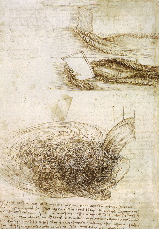
The great Renaissance artist, Leonardo Da Vinci, was one of the first
researchers in the field of fluid dynamics and turbulence. He used his
artistic abilities to document fluids in turbulent motion, the results
of which are shown opposite.
In his work, he uncovered a process similar to the bifurcations discussed in section 5.1.1. Eddies fragment into smaller and smaller eddies, resulting in turbulence. This is known as the period doubling route to chaos. Although turbulence looks very similar to other forms of bifurcatory behaviour, it is unclear as to whether the windows of order previously described can be seen.
Despite the avid interest of Leonardo and others, such as Lord Kelvin, turbulence remained a backwater field of study until recently, when chaos shed new light on the subject.
Turbulence is something that science has always had difficulty explaining, since it is very difficult to model. Water travelling down a pipe has no outside influences that could possibly induce turbulent motion, and yet, if the volume of water is high enough, turbulence appears, seemingly from nowhere.
One of the simplest ways to look at fluids that develop turbulent motion is a Taylor-Couette system, first studied at Cambridge by Geoffry Ingram Taylor during the 1920s. This, basically, consists of two cylinders, one inside the other. The outer cylinder remains stationary while the inner cylinder turns to create movement of the fluid in between.
The equations that explain fluid motion are called Navier-Stokes equations after Claude Navier (1785-1836) and George Stokes (1819-1903) who developed them independently. Being based on Newtons laws of motion, they are deterministic. As we have seen, this does not necessarily mean that it is a simple matter to make predictions. The Navier-Stokes equations are non-linear, meaning that there is a large potential for chaotic behaviour in the system. This has been demonstrated in section 5.1.2 using the simple mathematical population model xnext = x * l * (1 x).
When the water flow is slow, the Taylor-Couette System has few surprises. The flow is mainly in concentric circles around the axis of the cylinders. However, most of the fluid movement in nature is chaotic and as " laminar flow is not usually found in nature, it does not have much practical value."
As the speed of the inner cylinder increases, a secondary motion suddenly appears, superimposed upon the first. This motion has been described as "stacked Swiss rolls" that run horizontally to the vertical Taylor-Couette system. Increasing the speed yet further adds another, separate motion. The faster the system is run, the smaller the increase in speed needed to induce a new motion. Because of this, it would not be long before all possible motions were in action and, according to a Lev Landau theorem put forward in 1944, this was turbulence.
Since then, however, this idea has been challenged. Several scientists have been working with theories more in line with the mathematical model mentioned above. One researcher, Gerd Pfister of the University of Kiel, uncovered a period-doubling in fluid motion using a miniature (and therefore simpler) version of the Taylor-Couette system. According to Tom Mullin of the Clarendon Laboratory at Oxford, visual representations of this procedure are qualitatively the same as that of the simple differential equations described in section 5.1.1. The parallels between this system and Robert Mays bifurcations are immediately obvious. Analogies can be extended further, Mullin says, to situations such as chemical oscillators and lasers. This is another of the major features of chaos. There is a universality that crosses the borders of conventional disciplines.
Although turbulence is far from being understood, "mathematical ideas of chaos may have found a chink in the armour" of a mystery that lead British physicist, Horace Lamb, to say: